SpatialArtifacts Tutorial

Introduction

SpatialArtifacts is an R package that provides a data-driven a two-step workflow to identify, classify, and handle spatial artifacts in spatial transcriptomics data from multiple platforms including 10x Visium (Standard and HD). Broadly, the idea behind the package is we that combine median absolute deviation (MAD)-based outlier detection with morphological image processing to identify the artifacts. These artifacts, often appearing as areas of low gene/UMI counts or high mitochondrial ratio at tissue edges (edge artifacts) or in the interior (interior artifacts), can negatively impact downstream analyses. The methods are implemented as an R package within the Bioconductor framework, and is available from Bioconductor.

In the following, we provide an overview of the functionality in the package and we demonstrate how to apply the package on real-world datasets across different spatial transcriptomics platforms.

More details describing the method are available in our paper, available from bioRxiv.

Installation

The following code will install the latest release version of the SpatialArtifacts package from Bioconductor. Additional details are shown on Bioconductor.

Code

install.packages("BiocManager")
BiocManager::install("SpatialArtifacts")

The latest development version can also be installed from the devel version of Bioconductor or from GitHub.

Input data format

In the examples below, we assume the input data are provided as a SpatialExperiment Bioconductor object. In this case, the outputs are stored in the rowData of the SpatialExperiment object.

Platform Support

SpatialArtifacts is designed to work across multiple spatial transcriptomics platforms:

Standard Visium (55µm bins, hexagonal grid): ~5,000 spots per capture area
VisiumHD 16µm (16µm bins, square grid): ~480,000 bins per capture area
VisiumHD 8µm (8µm bins, square grid): ~1,920,000 bins per capture area

:::.::: {.callout-important}

The morphological detection framework automatically adapts to different grid arrangements, but parameter scaling is critical for optimal performance across platforms.

:::

Two key steps

The core philosophy is a two-step process: detect, and then classify. This separates the sensitive task of identifying all potential problem spots from the more nuanced task of deciding what to do with them.

The detection phase

In the first step, we use the detectEdgeArtifacts() function. Here, the goal is to identify all spots that could potentially be part of an artifact.

How does it work:

Outlier identification: Find spots with abnormally low QC metrics (e.g., sum_gene) using a Median Absolute Deviation (MAD) threshold.
Morphological cleaning: Apply sequential raster-based focal operations through focal_transformations():
1. 3×3 fill (my_fill): Fill spots completely surrounded by outliers
2. 5×5 outline (my_outline): Fill spots outlined by outliers in a larger 16-pixel perimeter
3. Star pattern (my_fill_star): Fill spots with outliers in all four cardinal directions (N, S, E, W)
4. Small cluster removal: Remove isolated normal regions below min_cluster_size threshold (default: 40 spots)
- Use 8-directional connectivity for connected component analysis
Cluster detection: Group these outliers into contiguous “problem areas” (problemAreas)
Edge identification: Evaluate whether clusters touch tissue boundaries using clumpEdges(). For each of the four borders (north, south, east, west), calculates the proportion of boundary spots belonging to each cluster. A cluster is classified as an edge artifact if this proportion meets or exceeds edge_threshold (default: 0.75, meaning ≥75% border coverage) on any single border direction

The output from this phase will add three raw columns to your spe object: _edge, _problem_id, and _problem_size

The classification phase

In the second step, we use the classifyEdgeArtifacts() function. Here the goal is to take the raw detections from the previous step and apply a clear, hierarchical logic to assign final labels.

How does it work:

Input: Requires the spe object processed by detectEdgeArtifacts()
Hierarchical Classification: Apply a 2×2 logic system based on Location and Size:
1. Location: Is the artifact an _edge_artifact (TRUE or FALSE) based on the detection step?
2. Size: Is the artifact’s _problem_size larger than min_spots (default: 20)?
Label Assignment: This logic produces five intuitive categories:
- "not_artifact" — High-quality spots
- "large_edge_artifact" — Large artifact cluster (> min_spots) touching the tissue edge
- "small_edge_artifact" — Small artifact cluster (≤ min_spots) touching the tissue edge
- "large_interior_artifact" — Large artifact cluster (> min_spots) located inside the tissue
- "small_interior_artifact" — Small artifact cluster (≤ min_spots) located inside the tissue

The output from this phase will add one classification column named _classification.

Helpful information on parameters

Tuning the parameters lets you adapt the workflow to different tissue types, data quality, and spatial transcriptomics platforms. The package uses a wrapper function that routes to platform-specific implementations.

Platform selection

CRITICAL FIRST STEP: Specify your platform using the platform parameter in detectEdgeArtifacts() function:

Platform	Function Call	Required Parameters
Standard Visium	`detectEdgeArtifacts(spe, platform="visium", ...)`	`shifted` (usually `TRUE`)
VisiumHD	`detectEdgeArtifacts(spe, platform="visiumhd", resolution="16um", ...)`	`resolution` (“8um” or “16um”)

Example use cases

Code

# Standard Visium (55µm hexagonal grid)
spe <- detectEdgeArtifacts(spe, platform = "visium", shifted = TRUE, ...)

# VisiumHD 16µm (square grid)
spe <- detectEdgeArtifacts(spe, platform = "visiumhd", resolution = "16um", ...)

# VisiumHD 8µm (square grid)
spe <- detectEdgeArtifacts(spe, platform = "visiumhd", resolution = "8um", ...)

Parameters for `detectEdgeArtifacts()`

The wrapper function accepts platform-specific parameters that are routed to the appropriate implementation.

For all platforms

platform (REQUIRED) – Character string: "visium" or "visiumhd" (case insensitive)
- Determines which platform-specific function to use
- No default value; must be explicitly specified for clarity
qc_metric (Default: "sum_gene") – Column name for QC metric used in outlier detection
- Common alternatives: "sum_umi", "detected", "nFeature"
- The function will auto-detect some common variants
samples (Default: "sample_id") – Column name for sample identifiers
- Each sample is processed independently
mad_threshold (Default: 3) – Sensitivity for detecting outliers
- Lower values (1.5–2) are more sensitive
- Higher values (3–4) are more conservative
name (Default: "edge_artifact") – Prefix for output column names
- Outputs: [name]_edge, [name]_problem_id, [name]_problem_size
verbose (Default: TRUE) – Print progress messages
keep_intermediate (Default: FALSE) – Retain intermediate outlier detection columns

For standard Visium

When platform = "visium", use:

edge_threshold (Default: 0.75) – Minimum proportion of a tissue boundary that must be occupied by outlier clusters (collectively) for those clusters to be classified as edge artifacts.

Important Behavior: The threshold is applied to the total coverage of all outlier clusters on each boundary direction (North, South, East, West). If multiple clusters collectively cover ≥ edge_threshold of a boundary, all clusters touching that boundary are classified as edge artifacts, even if no single cluster meets the threshold individually.

Example Scenario:
- North boundary contains 100 spots total
- Cluster A occupies 30 boundary spots (30% coverage)
- Cluster B occupies 50 boundary spots (50% coverage)
- Combined coverage: 80% ≥ 75% threshold
- Result: Both Cluster A and Cluster B are classified as edge artifacts
Rationale: Edge drying artifacts typically affect large, continuous regions along tissue boundaries. Multiple clusters on the same boundary often result from a single underlying technical failure (incomplete permeabilization) and should be treated as a unified artifact rather than independent events.

Tuning Guidance:
- Higher values (0.75–0.90): More conservative, captures only large-scale boundary failures
- Lower values (0.40–0.60): More sensitive, may flag smaller boundary-adjacent regions
- Very low values (<0.30): Aggressive, may misclassify biological low-expression zones as artifacts
min_cluster_size (Default: 40) – Minimum cluster size (in spots) for morphological cleaning during focal transformation steps
- Isolated “normal” regions smaller than this threshold within outlier areas will be filled in to create contiguous artifact regions
- For Standard Visium: 40 spots ≈ 0.12 mm² physical area
shifted (Default: FALSE) – Apply coordinate adjustment for hexagonal grid alignment
- Standard Visium typically requires shifted = TRUE when using array coordinates from Space Ranger.
- Set to FALSE if using pre-transformed pixel coordinates or for VisiumHD square grids.
- This corrects for the staggered arrangement of hexagonal spots
batch_var (Default: "both") – Determines grouping for MAD calculation
- Options: "sample_id", "slide", or "both"
- "both": Spots flagged as outliers if below threshold in either sample or slide grouping

For VisiumHD

When platform = "visiumhd", use:

resolution (REQUIRED) – Character string: "8um" or "16um"
- Specifies the bin size of your VisiumHD data
- This is mandatory for VisiumHD; the function will error if not provided
- Determines conversion from physical units (µm) to bins
buffer_width_um (Default: 80) – Buffer zone width in micrometers (physical units)
- Defines the edge region where artifacts are expected
- Automatically converted to bins based on resolution:
  - At 16µm resolution: 80 µm → 5 bins
  - At 8µm resolution: 80 µm → 10 bins
- Tuning guidance:
  - Increase (100-150 µm) for tissues with larger edge artifacts
  - Decrease (50-60 µm) for precise edge detection
min_cluster_area_um2 (Default: 1280) – Minimum cluster area in square micrometers (physical units)
- Clusters smaller than this will be filtered out during morphological cleaning
- Automatically converted to bins based on resolution:
  - At 16µm resolution: 1280 µm² → 5 bins (16×16 µm per bin)
  - At 8µm resolution: 1280 µm² → 20 bins (8×8 µm per bin)
- Physical consistency: Same area threshold gives different bin counts at different resolutions
- Default (1280 µm²) was calibrated for 16µm resolution
col_x and col_y (Default: "array_col", "array_row") – Column names for bin coordinates
- Important: These should be bin indices, not pixel coordinates
- Using bin indices is much more memory-efficient than pixel coordinates

Key Difference from Visium: VisiumHD parameters are specified in physical units (µm, µm²) rather than bin counts. This ensures consistency across resolutions while the algorithm handles the bin conversion internally.

Parameters for `classifyEdgeArtifacts()`

The classification step is platform-independent but requires appropriate parameter scaling.

min_spots (Default: 20) – CRITICAL PARAMETER: Threshold (in number of spots/bins) to distinguish "large" from "small" artifacts

Platform-Specific Scaling Required:

This parameter must be adjusted based on spatial resolution to represent equivalent physical artifact sizes:

Platform	Recommended `min_spots`	Physical Area	Scaling Factor
Standard Visium (55µm)	`20-40`	~0.06-0.12 mm²	Baseline (1×)
VisiumHD 16µm bins	`100-200`	~0.026-0.051 mm²	~6-10× Visium
VisiumHD 8µm bins	`400-800`	~0.026-0.051 mm²	~20-40× Visium

Automatic Scaling Formula:

min_spots_HD <- min_spots_visium × (55 / bin_size_µm)²

# Example: For min_spots = 30 on Standard Visium
# VisiumHD 16µm: 30 × (55/16)² ≈ 354 bins
# VisiumHD 8µm:  30 × (55/8)²  ≈ 1,420 bins

Why scaling matters: The same physical artifact (e.g., 0.1 mm² edge dryspot) will cover:

Standard Visium: ~33 spots
VisiumHD 16µm: ~390 bins
VisiumHD 8µm: ~1,560 bins

Without scaling, large VisiumHD artifacts would be incorrectly classified as “small.”

qc_metric (Default: "sum_umi") – QC metric column for validation (must exist but not directly used in classification logic)
samples (Default: "sample_id") – Sample ID column name
exclude_slides (Default: NULL) – Vector of slide IDs to exclude from edge classification
- Spots on these slides will have edge artifact status set to FALSE
name (Default: "edge_artifact") – Must match the name used in detectEdgeArtifacts()

Platform Comparison Summary

Feature	Standard Visium	VisiumHD
Grid Type	Hexagonal	Square
Requires `shifted`?	Yes (`TRUE`)	No (not used)
Resolution Parameter	Not applicable	Required (`"8um"` or `"16um"`)
Edge Detection Method	Morphological + boundary coverage	Buffer zone + morphological
Parameter Units	Spot counts	Physical units (µm, µm²)
Default `min_spots` (classify)	20-40	100-200 (16µm), 400-800 (8µm)
Typical Dataset Size	~5,000 spots	~480k bins (16µm), ~1.9M bins (8µm)

Understanding the output columns

After both functions, several columns are added to colData(spe):

*_edge – Raw detection: Is the spot in a cluster touching the tissue border? (TRUE/FALSE)
*_problem_id – Raw detection: ID of the problem area.
*_problem_size – Raw detection: Size (number of spots) of the problem area.
*_true_edges — Intermediate: Edge status after applying exclude_slides (used by classifyEdgeArtifacts()).
*_classification — Final classification: One of "not_artifact", "large_edge_artifact", "small_edge_artifact", "large_interior_artifact", or "small_interior_artifact".

Example: Standard Visium workflow

This package includes spe_vignette, a lightweight SpatialExperiment object derived from a human hippocampus Visium sample.

This vignette will load this raw-like object and run the full SpatialArtifacts workflow on it live.

Note: To meet package size requirements (< 5MB), this object has been subset (e.g., to coding genes) and sparsified, but no artifact detection has been run. We will perform those steps now.

Data preparation: converting to dense matrix

The underlying spatial clustering functions in this package currently require a dense matrix to perform coordinate-based calculations. We must first convert the sparse counts assay in our spe_vignette object to a standard (dense) matrix.

Code

data(spe_vignette)
cat("Loaded data dimensions:", dim(spe_vignette), "\n")
#> Loaded data dimensions: 12971 4965

assay(spe_vignette, "counts") <- as.matrix(assay(spe_vignette, "counts"))
names(colData(spe_vignette))[names(colData(spe_vignette)) == "sum"] <- "sum_umi"

spe_detected <- detectEdgeArtifacts(
  spe_vignette,
  platform = "visium", # IMPORTANT: Specify Standard Visium platform
  qc_metric = "sum_umi",
  samples = "sample_id",
  shifted = TRUE, # Hexagonal grid coordinate adjustment
  batch_var = "sample_id",
  mad_threshold = 3,
  edge_threshold = 0.75,
  name = "edge_artifact"
)
#> Detecting edges...
#>   Sample V11L05-335_C1: 74 edge spots detected
#> Finding problem areas...
#> Removed intermediate columns: lg10_sum_umi, sum_umi_3MAD_outlier_sample, sum_umi_3MAD_outlier_binary
#> Edge artifact detection completed!
#>   Total edge spots: 74
#>   Total problem area spots: 78

cat("\n=== RESULTS ===\n")
#> 
#> === RESULTS ===
table(Edge_Detected = spe_detected$edge_artifact_edge)
#> Edge_Detected
#> FALSE  TRUE 
#>  4891    74

# Classification with Standard Visium parameters
spe_classified <- classifyEdgeArtifacts(
  spe_detected,
  min_spots = 20,
  name = "edge_artifact"
)
#> Classifying artifacts spots...
#> Classification added: edge_artifact_classification
#> 
#> Classification summary:
#>   not_artifact: 4887 spots
#>   small_edge_artifact: 74 spots
#>   small_interior_artifact: 4 spots

cat("\n=== Classification Results ===\n")
#> 
#> === Classification Results ===
table(spe_classified$edge_artifact_classification)
#> 
#>            not_artifact     small_edge_artifact small_interior_artifact 
#>                    4887                      74                       4

VisiumHD Workflow Example

For VisiumHD data, the workflow is identical except for parameter scaling. Here’s a complete example showing how to adapt parameters for VisiumHD:

VisiumHD 16µm Resolution Example

Code

# This is a pseudo-example demonstrating VisiumHD 16µm workflow
# Assumes you have loaded a VisiumHD SpatialExperiment object as 'spe_hd16'

# Step 1: Ensure required QC metrics are calculated
library(scuttle)
spe_hd16 <- addPerCellQCMetrics(spe_hd16)

# Step 2: Detection Phase - VisiumHD uses square grid (no 'shifted' needed)
spe_hd16_detected <- detectEdgeArtifacts(
  spe_hd16,
  platform = "visiumhd", # Specify VisiumHD platform
  resolution = "16um", # REQUIRED for VisiumHD
  qc_metric = "sum_umi", # or "sum" depending on your colData
  samples = "sample_id",
  buffer_width_um = 100, # VisiumHD-specific parameter
  mad_threshold = 2.5,
  edge_threshold = 0.75,
  name = "edge_artifact"
)

# Step 3: Classification Phase - CRITICAL: Scale min_spots for VisiumHD resolution
# For 16µm bins, use ~6-10× the Standard Visium threshold
min_spots_16um <- 30 * (55 / 16)^2 # ≈ 354 bins

spe_hd16_classified <- classifyEdgeArtifacts(
  spe_hd16_detected,
  qc_metric = "sum_umi",
  min_spots = round(min_spots_16um), # ~350 bins
  name = "edge_artifact"
)

# Visualization (same approach as Standard Visium)
table(spe_hd16_classified$edge_artifact_classification)

VisiumHD 8µm Resolution Example

Code

# This is a pseudo-example demonstrating VisiumHD 8µm workflow
# Assumes you have loaded a VisiumHD 8µm SpatialExperiment object as 'spe_hd8'

# Step 1: QC metrics
spe_hd8 <- addPerCellQCMetrics(spe_hd8)

# Step 2: Detection Phase
spe_hd8_detected <- detectEdgeArtifacts(
  spe_hd8,
  platform = "visiumhd", # Specify VisiumHD platform
  resolution = "8um", # REQUIRED: Specify 8µm resolution
  qc_metric = "sum_umi",
  samples = "sample_id",
  buffer_width_um = 100, # Buffer zone in micrometers
  mad_threshold = 2.5,
  edge_threshold = 0.75,
  name = "edge_artifact"
)

# Step 3: Classification with 8µm-appropriate threshold
# For 8µm bins, use ~20-40× the Standard Visium threshold
min_spots_8um <- 30 * (55 / 8)^2 # ≈ 1,420 bins

spe_hd8_classified <- classifyEdgeArtifacts(
  spe_hd8_detected,
  qc_metric = "sum_umi",
  min_spots = round(min_spots_8um), # ~1,400 bins
  name = "edge_artifact"
)

table(spe_hd8_classified$edge_artifact_classification)

Key VisiumHD Considerations

Platform-Specific Function Calls:

Platform	Function Call	Required Parameters
Standard Visium	`detectEdgeArtifacts(..., platform="visium")`	`shifted=TRUE`
VisiumHD 16µm	`detectEdgeArtifacts(..., platform="visiumhd", resolution="16um")`	`resolution`
VisiumHD 8µm	`detectEdgeArtifacts(..., platform="visiumhd", resolution="8um")`	`resolution`

Parameter Recommendations by Platform:

Parameter	Standard Visium	VisiumHD 16µm	VisiumHD 8µm
`platform`	`"visium"`	`"visiumhd"`	`"visiumhd"`
`resolution`	N/A (not used)	`"16um"`	`"8um"`
`shifted`	`TRUE`	N/A (handled internally)	N/A
`buffer_width_um`	N/A	`100` (default)	`100` (default)
`mad_threshold`	1.5-3.0	2.0-3.0	2.0-3.0
`min_spots` (classify)	20-40	100-200	400-800
Grid Type	Hexagonal	Square	Square

Visualization: QC Metrics and Detection Results

We’ll create a comprehensive visualization showing QC metrics, detection results, and detailed cluster information:

Code

library(SpatialExperiment)
library(patchwork)

plot_data <- as.data.frame(colData(spe_classified))
plot_data <- cbind(plot_data, as.data.frame(spatialCoords(spe_classified)))
plot_data_in_tissue <- plot_data[plot_data$in_tissue, ]

base_theme <- theme_void() +
  theme(
    plot.title = element_text(size = 12, hjust = 0.5),
    legend.position = "right"
  )

# Plot 1: UMI Counts
p1 <- ggplot(plot_data_in_tissue, aes(
  x = pxl_col_in_fullres, y = pxl_row_in_fullres,
  color = log10(sum_umi + 1)
)) +
  geom_point(size = 0.5) +
  scale_color_viridis_c(name = "log10(UMI)") +
  ggtitle("A. UMI Counts") +
  base_theme +
  coord_fixed()

# Plot 2: Detected Genes
if ("detected" %in% names(plot_data_in_tissue)) {
  p2 <- ggplot(plot_data_in_tissue, aes(
    x = pxl_col_in_fullres, y = pxl_row_in_fullres,
    color = detected
  )) +
    geom_point(size = 0.5) +
    scale_color_viridis_c(name = "Genes", option = "plasma") +
    ggtitle("B. Detected Genes") +
    base_theme +
    coord_fixed()
} else {
  p2 <- ggplot() +
    theme_void() +
    ggtitle("B. Detected Genes (Data N/A)")
}

# Plot 3: Raw Detection (Any Problem Area)
if ("edge_artifact_problem_id" %in% names(plot_data_in_tissue)) {
  p3 <- ggplot(plot_data_in_tissue, aes(
    x = pxl_col_in_fullres, y = pxl_row_in_fullres,
    color = !is.na(edge_artifact_problem_id)
  )) +
    geom_point(size = 0.5) +
    scale_color_manual(
      values = c("FALSE" = "lightgray", "TRUE" = "red"),
      name = "Problem?"
    ) +
    ggtitle("C. Raw Detection (All Problem Areas)") +
    base_theme +
    coord_fixed()
} else {
  p3 <- ggplot() +
    theme_void() +
    ggtitle("C. Raw Detection (Data N/A)")
}

# Plot 4: Cluster IDs
if ("edge_artifact_problem_id" %in% names(plot_data_in_tissue)) {
  plot_data_in_tissue$cluster_display <- NA

  has_cluster <- !is.na(plot_data_in_tissue$edge_artifact_problem_id)
  plot_data_in_tissue$cluster_display[has_cluster] <-
    plot_data_in_tissue$edge_artifact_problem_id[has_cluster]

  n_clusters <- length(unique(plot_data_in_tissue$cluster_display[has_cluster]))

  p4 <- ggplot(plot_data_in_tissue, aes(
    x = pxl_col_in_fullres, y = pxl_row_in_fullres,
    color = cluster_display
  )) +
    geom_point(size = 0.5) +
    scale_color_discrete(name = "Cluster ID", na.value = "lightgray") +
    ggtitle(paste0("D. Problem Area Clusters (n=", n_clusters, ")")) +
    base_theme +
    coord_fixed() +
    theme(
      legend.key.size = unit(0.3, "cm"),
      legend.text = element_text(size = 8)
    )
} else {
  p4 <- ggplot() +
    theme_void() +
    ggtitle("D. Cluster IDs (Data N/A)")
}

# Plot 5: Edge vs Interior Separation
if ("edge_artifact_edge" %in% names(plot_data_in_tissue)) {
  plot_data_in_tissue$artifact_type <- "Normal"

  # Mark edge artifacts
  plot_data_in_tissue$artifact_type[plot_data_in_tissue$edge_artifact_edge] <- "Edge Artifact"

  # Mark interior problem areas (not edges)
  interior_mask <- !is.na(plot_data_in_tissue$edge_artifact_problem_id) &
    !plot_data_in_tissue$edge_artifact_edge
  plot_data_in_tissue$artifact_type[interior_mask] <- "Interior Problem"

  p5 <- ggplot(plot_data_in_tissue, aes(
    x = pxl_col_in_fullres, y = pxl_row_in_fullres,
    color = artifact_type
  )) +
    geom_point(size = 0.5) +
    scale_color_manual(
      values = c(
        "Normal" = "lightgray",
        "Edge Artifact" = "red",
        "Interior Problem" = "blue"
      ),
      name = "Artifact Type"
    ) +
    ggtitle("E. Edge vs Interior Distinction") +
    base_theme +
    coord_fixed()
} else {
  p5 <- ggplot() +
    theme_void() +
    ggtitle("E. Edge vs Interior (Data N/A)")
}

# Plot 6: Final Hierarchical Classification
if ("edge_artifact_classification" %in% names(plot_data_in_tissue)) {
  p6 <- ggplot(plot_data_in_tissue, aes(
    x = pxl_col_in_fullres, y = pxl_row_in_fullres,
    color = edge_artifact_classification
  )) +
    geom_point(size = 0.5) +
    scale_color_manual(
      values = c(
        "not_artifact" = "lightgray",
        "large_edge_artifact" = "red",
        "small_edge_artifact" = "orange",
        "large_interior_artifact" = "blue",
        "small_interior_artifact" = "cyan"
      ),
      name = "Final Class",
      na.value = "grey50"
    ) +
    ggtitle("F. Final Hierarchical Classification") +
    base_theme +
    coord_fixed()
} else {
  p6 <- ggplot() +
    theme_void() +
    ggtitle("F. Final Classification (Data N/A)")
}

# Combine all plots in a 3x2 layout
(p1 | p2) / (p3 | p4) / (p5 | p6)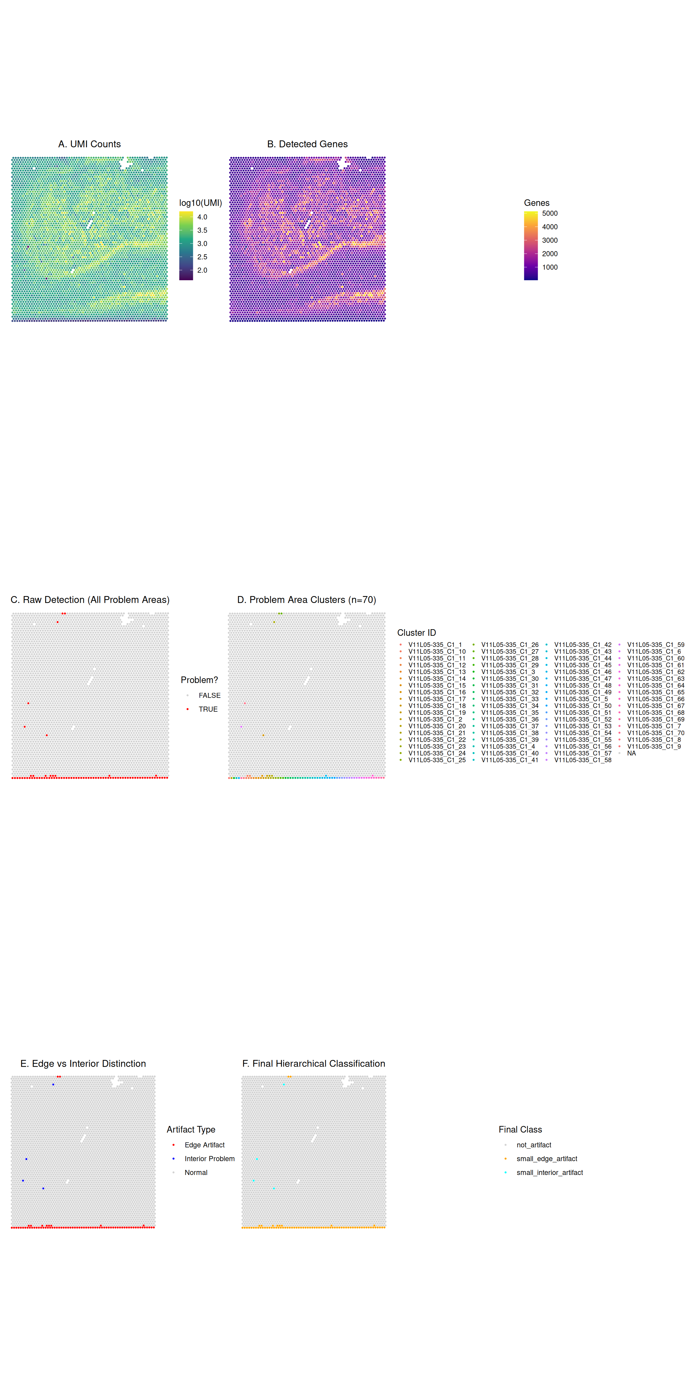

Classification Summary

Let’s examine the enhanced classification system:

Code

cat("--- Final Classification Summary (`edge_artifact_classification`) ---\n")
#> --- Final Classification Summary (`edge_artifact_classification`) ---
# Use the 'spe_classified' object we created in the step above
final_summary <- table(spe_classified$edge_artifact_classification)
print(final_summary)
#> 
#>            not_artifact     small_edge_artifact small_interior_artifact 
#>                    4887                      74                       4

final_pct <- round(100 * final_summary / sum(final_summary), 2)
final_df <- data.frame(
  Classification = names(final_summary),
  Count = as.numeric(final_summary),
  Percentage = as.numeric(final_pct)
)
print(final_df)
#>            Classification Count Percentage
#> 1            not_artifact  4887      98.43
#> 2     small_edge_artifact    74       1.49
#> 3 small_interior_artifact     4       0.08
cat("\n\n")

cat("--- Raw Edge Detection Summary (`edge_artifact_edge`) ---\n")
#> --- Raw Edge Detection Summary (`edge_artifact_edge`) ---
# Use the 'spe_classified' object and the new column name
edge_summary <- table(spe_classified$edge_artifact_edge)
print(edge_summary)
#> 
#> FALSE  TRUE 
#>  4891    74

edge_pct <- round(100 * edge_summary / sum(edge_summary), 2)
edge_df <- data.frame(
  Flagged_As_Edge = names(edge_summary),
  Count = as.numeric(edge_summary),
  Percentage = as.numeric(edge_pct)
)
print(edge_df)
#>   Flagged_As_Edge Count Percentage
#> 1           FALSE  4891      98.51
#> 2            TRUE    74       1.49

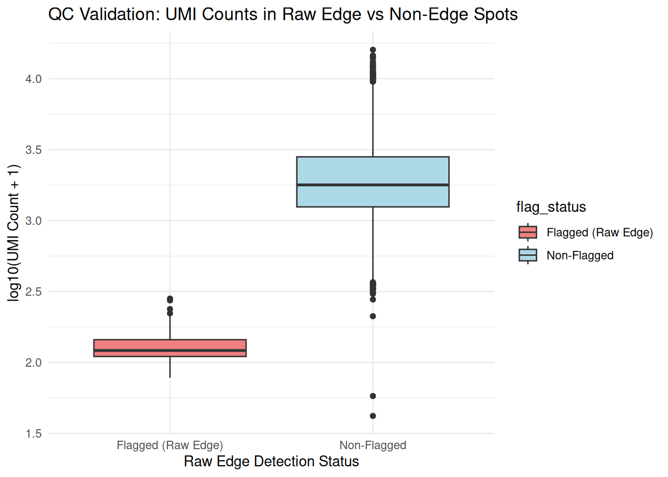
Quality Control Validation

Finally, let’s validate that flagged spots have lower quality metrics:

Code

in_tissue_data <- spe_classified[, spe_classified$in_tissue]

qc_data <- data.frame(
  sum_umi = in_tissue_data$sum_umi,
  detected_genes = in_tissue_data$detected,
  flagged = in_tissue_data$edge_artifact_edge
)

# --- Calculate Median Differences ---
flagged_umi <- median(qc_data$sum_umi[qc_data$flagged], na.rm = TRUE)
nonflagged_umi <- median(qc_data$sum_umi[!qc_data$flagged], na.rm = TRUE)

flagged_gene <- median(qc_data$detected_genes[qc_data$flagged], na.rm = TRUE)
nonflagged_gene <- median(qc_data$detected_genes[!qc_data$flagged], na.rm = TRUE)

cat("QC Validation Results (comparing raw edge detection flag):\n")
#> QC Validation Results (comparing raw edge detection flag):
cat("Flagged spots - Median UMI:", round(flagged_umi), "\n")
#> Flagged spots - Median UMI: 120
cat("Non-flagged spots - Median UMI:", round(nonflagged_umi), "\n")
#> Non-flagged spots - Median UMI: 1784
cat("UMI difference:", round(nonflagged_umi - flagged_umi), "\n\n")
#> UMI difference: 1664

cat("Flagged spots - Median Detected Genes:", round(flagged_gene), "\n")
#> Flagged spots - Median Detected Genes: 106
cat("Non-flagged spots - Median Detected Genes:", round(nonflagged_gene), "\n")
#> Non-flagged spots - Median Detected Genes: 1019
cat("Gene difference:", round(nonflagged_gene - flagged_gene), "\n")
#> Gene difference: 912

qc_data$flag_status <- ifelse(qc_data$flagged, "Flagged (Raw Edge)", "Non-Flagged")

validation_plot <- ggplot(qc_data, aes(x = flag_status, y = log10(sum_umi + 1), fill = flag_status)) +
  geom_boxplot() +
  scale_fill_manual(values = c("Flagged (Raw Edge)" = "lightcoral", "Non-Flagged" = "lightblue")) +
  labs(
    title = "QC Validation: UMI Counts in Raw Edge vs Non-Edge Spots",
    x = "Raw Edge Detection Status", y = "log10(UMI Count + 1)"
  ) +
  theme_minimal()

print(validation_plot)

Filtering Out Problematic Spots (Optional)

Based on the new classifications, users can make informed decisions about filtering. For example, you might decide to remove all edge artifacts (both large and small) while keeping interior artifacts for further review.

Here’s how you can filter the SpatialExperiment object to remove all spots classified as both "large_edge_artifact" or "small_edge_artifact":

Code

if ("edge_artifact_classification" %in% names(colData(spe_classified))) {
  spots_to_keep <- !spe_classified$edge_artifact_classification %in%
    c("large_edge_artifact", "small_edge_artifact")
  spe_filtered <- spe_classified[, spots_to_keep]
  cat("Original number of spots:", ncol(spe_classified), "\n")
  cat("Number of spots after filtering:", ncol(spe_filtered), "\n")
} else {
  cat("Classification column not found. Filtering step skipped.\n")
}
#> Original number of spots: 4965 
#> Number of spots after filtering: 4891

Code

plot_data_before <- as.data.frame(colData(spe_classified))
coords_mat <- spatialCoords(spe_classified)
plot_data_before <- cbind(plot_data_before, as.data.frame(coords_mat))
plot_data_before_in_tissue <- plot_data_before[plot_data_before$in_tissue, ]

plot_data_after <- as.data.frame(colData(spe_filtered))
if (ncol(spe_filtered) > 0) {
  coords_mat_after <- spatialCoords(spe_filtered)
  plot_data_after <- cbind(plot_data_after, as.data.frame(coords_mat_after))
}

base_theme <- theme_void() +
  theme(
    plot.title = element_text(size = 12, hjust = 0.5),
    legend.position = "right"
  )

p1_umi_before <- ggplot(plot_data_before_in_tissue, aes(x = pxl_col_in_fullres, y = pxl_row_in_fullres, color = log10(sum_umi + 1))) +
  geom_point(size = 0.5) +
  scale_color_viridis_c(name = "log10(UMI)") +
  ggtitle("UMI Counts (Before Filtering)") +
  base_theme +
  coord_fixed()

if (ncol(spe_filtered) > 0) {
  p2_umi_after <- ggplot(plot_data_after, aes(x = pxl_col_in_fullres, y = pxl_row_in_fullres, color = log10(sum_umi + 1))) +
    geom_point(size = 0.5) +
    scale_color_viridis_c(name = "log10(UMI)") +
    ggtitle("UMI Counts (After Filtering)") +
    base_theme +
    coord_fixed()
} else {
  p2_umi_after <- ggplot() +
    theme_void() +
    ggtitle("UMI Counts (After Filtering - No Spots)")
}

p3_class_before <- ggplot(plot_data_before_in_tissue, aes(x = pxl_col_in_fullres, y = pxl_row_in_fullres, color = edge_artifact_classification)) +
  geom_point(size = 0.5) +
  scale_color_manual(
    values = c(
      "not_artifact" = "lightgray",
      "large_edge_artifact" = "red",
      "small_edge_artifact" = "orange",
      "large_interior_artifact" = "blue",
      "small_interior_artifact" = "cyan"
    ),
    name = "Final Class",
    na.value = "grey50",
    drop = FALSE
  ) +
  ggtitle("Classification (Before Filtering)") +
  base_theme +
  coord_fixed()

if (ncol(spe_filtered) > 0) {
  p4_class_after <- ggplot(plot_data_after, aes(x = pxl_col_in_fullres, y = pxl_row_in_fullres, color = edge_artifact_classification)) +
    geom_point(size = 0.5) +
    scale_color_manual(
      values = c(
        "not_artifact" = "lightgray",
        "large_edge_artifact" = "red",
        "small_edge_artifact" = "orange",
        "large_interior_artifact" = "blue",
        "small_interior_artifact" = "cyan"
      ),
      name = "Final Class",
      na.value = "grey50",
      drop = FALSE
    ) +
    ggtitle("Classification (After Filtering)") +
    base_theme +
    coord_fixed()
} else {
  p4_class_after <- ggplot() +
    theme_void() +
    ggtitle("Classification (After Filtering - No Spots)")
}

combined_filtering_plot_2x2 <- (p1_umi_before | p2_umi_after) / (p3_class_before | p4_class_after)
print(combined_filtering_plot_2x2)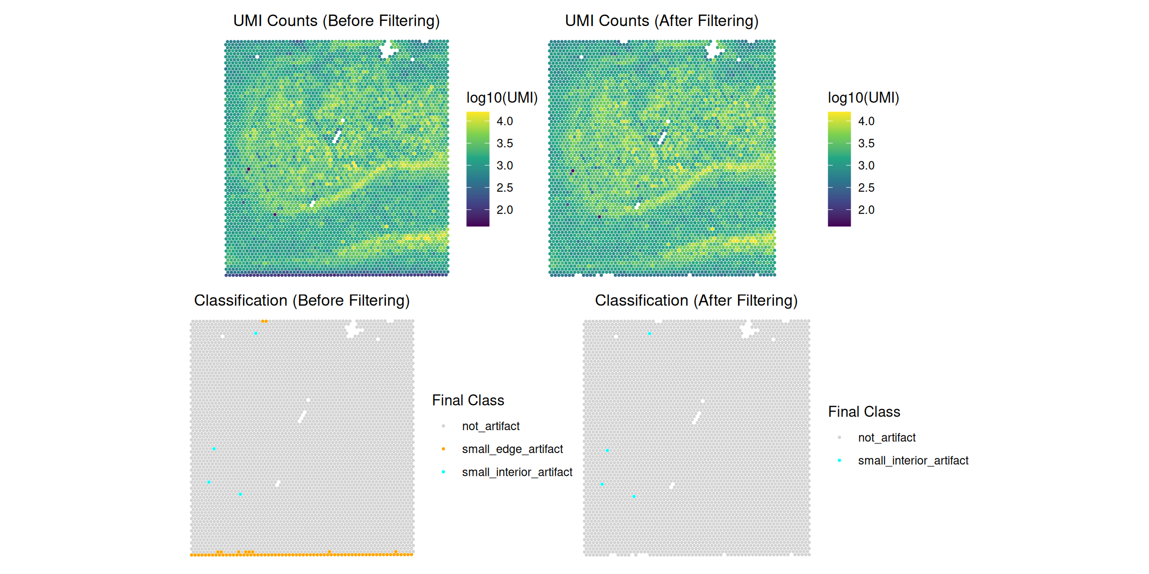

Conclusion

This vignette demonstrated the SpatialArtifacts workflow across multiple spatial transcriptomics platforms. Specifically, it showed:

Standard Visium workflow: Complete example using the included hippocampus dataset
VisiumHD adaptation: How to properly scale parameters for 16µm and 8µm resolution data
Platform-specific considerations: Grid arrangement, parameter scaling formulas, and typical artifact sizes
Visualization: Display hierarchical classification results alongside QC metrics
Classification logic: Distinguish between edge vs. interior and large vs. small artifacts
Validation: Flagged spots show significantly lower molecular capture

Key Takeaways for Multi-Platform Usage:

Grid Structure: Standard Visium uses hexagonal grids (shifted = TRUE), while VisiumHD uses square grids (shifted = FALSE)
Critical Parameter Scaling: The min_spots threshold in classifyEdgeArtifacts() must scale with spatial resolution:
- Use the formula: min_spots_HD = min_spots_visium × (55 / bin_size)²
- Without scaling, artifacts will be incorrectly classified by size
Morphological Framework: The same detection logic works across platforms, automatically adapting to different grid arrangements
Physical Consistency: Scaled parameters ensure that “large” and “small” artifact classifications represent equivalent physical sizes regardless of platform

Overall, SpatialArtifacts provides a unified, platform-agnostic framework for detecting and classifying spatial artifacts, enabling consistent quality control across the evolving spatial transcriptomics technology landscape.

Session Information

Code

sessionInfo()
#> R version 4.5.2 (2025-10-31)
#> Platform: x86_64-pc-linux-gnu
#> Running under: Ubuntu 24.04.3 LTS
#> 
#> Matrix products: default
#> BLAS:   /usr/lib/x86_64-linux-gnu/openblas-pthread/libblas.so.3 
#> LAPACK: /usr/lib/x86_64-linux-gnu/openblas-pthread/libopenblasp-r0.3.26.so;  LAPACK version 3.12.0
#> 
#> locale:
#>  [1] LC_CTYPE=C.UTF-8       LC_NUMERIC=C           LC_TIME=C.UTF-8       
#>  [4] LC_COLLATE=C.UTF-8     LC_MONETARY=C.UTF-8    LC_MESSAGES=C.UTF-8   
#>  [7] LC_PAPER=C.UTF-8       LC_NAME=C              LC_ADDRESS=C          
#> [10] LC_TELEPHONE=C         LC_MEASUREMENT=C.UTF-8 LC_IDENTIFICATION=C   
#> 
#> time zone: UTC
#> tzcode source: system (glibc)
#> 
#> attached base packages:
#> [1] stats4    stats     graphics  grDevices utils     datasets  methods  
#> [8] base     
#> 
#> other attached packages:
#>  [1] dplyr_1.2.0                 patchwork_1.3.2            
#>  [3] ggplot2_4.0.2               SpatialArtifacts_0.99.0    
#>  [5] SpatialExperiment_1.20.0    SingleCellExperiment_1.32.0
#>  [7] SummarizedExperiment_1.40.0 Biobase_2.70.0             
#>  [9] GenomicRanges_1.62.1        Seqinfo_1.0.0              
#> [11] IRanges_2.44.0              S4Vectors_0.48.0           
#> [13] BiocGenerics_0.56.0         generics_0.1.4             
#> [15] MatrixGenerics_1.22.0       matrixStats_1.5.0          
#> 
#> loaded via a namespace (and not attached):
#>  [1] SparseArray_1.10.8  scuttle_1.20.0      lattice_0.22-7     
#>  [4] digest_0.6.39       magrittr_2.0.4      evaluate_1.0.5     
#>  [7] grid_4.5.2          RColorBrewer_1.1-3  fastmap_1.2.0      
#> [10] jsonlite_2.0.0      Matrix_1.7-4        viridisLite_0.4.3  
#> [13] scales_1.4.0        codetools_0.2-20    abind_1.4-8        
#> [16] cli_3.6.5           rlang_1.1.7         XVector_0.50.0     
#> [19] withr_3.0.2         DelayedArray_0.36.0 yaml_2.3.12        
#> [22] S4Arrays_1.10.1     tools_4.5.2         beachmat_2.26.0    
#> [25] parallel_4.5.2      BiocParallel_1.44.0 vctrs_0.7.1        
#> [28] R6_2.6.1            lifecycle_1.0.5     magick_2.9.1       
#> [31] pkgconfig_2.0.3     terra_1.8-93        pillar_1.11.1      
#> [34] gtable_0.3.6        glue_1.8.0          Rcpp_1.1.1         
#> [37] xfun_0.56           tibble_3.3.1        tidyselect_1.2.1   
#> [40] knitr_1.51          farver_2.1.2        rjson_0.2.23       
#> [43] htmltools_0.5.9     labeling_0.4.3      rmarkdown_2.30     
#> [46] compiler_4.5.2      S7_0.2.1

Introduction

Installation

Input data format

Platform Support

Two key steps

The detection phase

The classification phase

Helpful information on parameters

Platform selection

Example use cases

Parameters for detectEdgeArtifacts()

For all platforms

For standard Visium

For VisiumHD

Parameters for classifyEdgeArtifacts()

Platform Comparison Summary

Understanding the output columns

Example: Standard Visium workflow

Data preparation: converting to dense matrix

VisiumHD Workflow Example

VisiumHD 16µm Resolution Example

VisiumHD 8µm Resolution Example

Key VisiumHD Considerations

Visualization: QC Metrics and Detection Results

Classification Summary

Quality Control Validation

Filtering Out Problematic Spots (Optional)

Conclusion

Session Information

Parameters for `detectEdgeArtifacts()`

Parameters for `classifyEdgeArtifacts()`